
−1 ≤ r ≤ 1
but it is not based on ranking the data but uses the actual data values. We will first introduce the idea of 'covariance'.
Worked Examples
| Pupil | A | B | C | D | E | F | G | H | I | J |
| Maths mark (out of 30) x | 20 | 23 | 8 | 29 | 14 | 11 | 11 | 20 | 17 | 17 |
| Physics mark (out of 40) y | 30 | 35 | 21 | 33 | 33 | 26 | 22 | 31 | 33 | 36 |
Is there a connection between the marks gained by ten pupils, A, B, C ..., J in Maths and Physics tests?
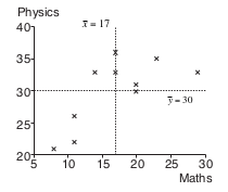
As a starting point, plot the marks as a scatter diagram.
The areas in the bottom right and top left of the graph are largely vacant so there is a tendency for the points to run from bottom left to top right.
Now calculate the means,
\overline{x} = \frac{170}{10} = 17
and
\overline{y} = \frac{300}{10} = 30
Using the means to divide the graph into four shows this tendency clearly.
The problem though is to find a way to measure how strong the tendency is.
We can attempt to quantify the tendency to go from bottom left to top right by evaluating
the expression
which is known as the covariance and denoted by cov(X,Y) or s_{xy}. For shorthand it is normally written as
\frac{1}{n}\sum_{\ }^{\ }\left(x-\overline{x}\right)\left(y-\overline{y}\right)
where the summation over i is assumed.
The points in the top right have x and y values greater than \overline{x} and \overline{y} respectively, so x - \overline{x} and y - \overline{y} are both positive and so is the product \left(x-\overline{x}\right)\left(y-\overline{y}\right).
Those in the bottom left have values less than \overline{x} and \overline{y} , so x - \overline{x} and y - \overline{y} are both negative and again the product \left(x-\overline{x}\right)\left(y-\overline{y}\right) is positive.
Points in the other two areas have one of x - \overline{x} and y - \overline{y} positive and the other negative, so x - \overline{x} and y - \overline{y} is negative.
The \frac{1}{n} factor accounts for the fact that the number of points will affect the value of the covariance.
In the example above, most of the points give positive values of \left(x-\overline{x}\right)\left(y-\overline{y}\right).
There is another form of the expression for covariance which is easier to use in calculations.
| \frac{1}{n}\sum_{\ }^{\ }\left(x-\overline{x}\right)\left(y-\overline{y}\right) | = \frac{1}{n}\sum_{\ }^{\ }\left(xy-\overline{x}y-x\overline{y}+\overline{xy}\right) | |
| = \frac{1}{n}\left(\sum_{\ }^{\ }xy-\sum_{\ }^{\ }\overline{x}y-\sum_{\ }^{\ }x\overline{y}+\sum_{\ }^{\ }\overline{xy}\right) | ||
| = \frac{1}{n}\left(\sum_{\ }^{\ }xy-\overline{x}\sum_{\ }^{\ }y-\overline{y}\sum_{\ }^{\ }x+n\overline{xy}\right) | ||
| = \frac{1}{n}\left(\sum_{\ }^{\ }xy-\overline{x}n\overline{y}-\overline{y}n\overline{x}+n\overline{xy}\right) | since \overline{y}=\frac{\sum_{\ }^{\ }y}{n},\ \overline{x}=\frac{\sum_{\ }^{\ }x}{n} | |
| = \frac{1}{n}\left(\sum_{\ }^{\ }xy-n\overline{xy}\right) |
Thus
The right hand side is quicker to evaluate. For the example on page 15, this form of the expression is usually used when calculating covariance.
| s_{xy} | = \frac{1}{10}\Sigma\ xy-17\times30 |
| = \frac{1}{10}\times5313-510 | |
| = 21.3 |
( Σ xy is a function available on calculators with LR mode.)
The fact that s_{xy} > 0 indicates that the points follow a trend with a positive slope. The size of the number, however, conveys little as it can easily be altered by a change of scale. The following examples show this.
Find the covariance for the following data.
| Height (m) x | 1.60 | 1.64 | 1.71 |
| Weight (kg) y | 53 | 57 | 60 |
| s_{xy} | = \frac{1}{3}\times280.88-\frac{170}{3}\times\frac{4.95}{3} |
| = 0.126 |
| Height (cm) x | 160 | 164 | 171 |
| Weight (kg) y | 53 | 57 | 60 |
| s_{xy} | = \frac{1}{3}\times28088-\frac{170}{3}\times\frac{495}{3} |
| = 12.\dot{6} |
You can, of course, get quite different values by measuring in pounds and inches or kg and feet, etc. They will all be positive but their sizes will not convey useful information.
\frac{x-\overline{x}}{s_x}
will give the same answer regardless of the units or scale involved. The quantity
\frac{1}{n}\sum_{\ }^{\ }\left(\frac{x-\overline{x}}{s_x}\right)\left(\frac{y-\overline{y}}{s_y}\right)
can therefore be relied on to produce a value with more meaning than the covariance.
Since
\frac{1}{n}\sum_{\ }^{\ }\left(\frac{x-\overline{x}}{s_x}\right)\left(\frac{y-\overline{y}}{s_y}\right)=\frac{\frac{1}{n}\text{Σ}xy-\overline{xy}}{s_xs_y}
and the latter is easier to evaluate, Pearson's product moment correlation coefficient is often given as
where
s_x=\sqrt{\frac{1}{n}\text{Σ}x^2-\overline{x}^2} and s_x=\sqrt{\frac{1}{n}\text{Σ}y^2-\overline{y}^2}
(Note that r is a function given on calculators with LR mode.)
Returning to the Worked Example above:
| Pupil | A | B | C | D | E | F | G | H | I | J |
| Maths mark (out of 30) x | 20 | 23 | 8 | 29 | 14 | 11 | 11 | 20 | 17 | 17 |
| Physics mark (out of 40) y | 30 | 35 | 21 | 33 | 33 | 26 | 22 | 31 | 33 | 36 |
r = \frac{\frac{1}{10} × 5313 - 17 × 30}{s_x × s_y}
s_x = \sqrt{\frac{1}{10} × 3250 - 17^2} = \sqrt{36} = 6
s_y = \sqrt{\frac{1}{10} × 9250 - 30^2} = \sqrt{25} = 5
| ⇒ | r | = \frac{531.3 - 510}{6 × 5} |
| = 0.71 |
A group of twelve children participated in a psychological study designed to assess the relationship, if any, between age, x years, and average total sleep time (ATST), y minutes. To obtain a measure for ATST, recordings were taken on each child on five consecutive nights and then averaged. The results obtained are shown in the table.

Calculate the value of the product moment correlation coefficient between x and y.
Assess the statistical significance of your value and interpret your results.
Use the formula
s_{xy} = \frac{1}{n}\text{Σ}xy-\overline{xy}
when \overline{x} = \frac{108}{12} = 9 and \overline{y} = \frac{6372}{12} = 531
Thus s_{xy} = \frac{1}{12}(56825.4) - 9 × 531 = -43.55
Also
s_x = \sqrt{\frac{1}{12} × 1060.1 - 9^2} ≈ 2.7096
s_y = \sqrt{\frac{1}{12} × 3396942 - 531^2} ≈ 33.4290
Hence
r = \frac{-43.55}{2.7096 × 33.4290} ≈ -0.481
Exercises
