
If you play ten games of table tennis against an opponent who, from past experience, you know only has a chance of winning a game with you, how many games do you expect him to win?
Most people would reply 'two' and would argue that since the opponent wins on average of the games he can expect to be successful in × 10 = 2 .
Another way of writing this would be to say, if X ~ B(10, ), what is the value of E(X) where E(X) means the expected value of X? The answer then is E(X) = 10 × = 2.
In general, if X ~ B (n, p) , then the expected value of X is given by
The formal proof of this result requires some work from pure maths, and in particular uses the result that
\binom{n}{r} = \frac{n!}{r!(n - r)!}
The variance of X is given by
Worked Examples
A biased die is thrown thirty times and the number of sixes seen is eight. If the die is thrown a further twelve times find:
the probability that a six will occur exactly twice;
Show meLet X be defined by 'the number of sixes seen in twelve throws'.
Then X ~ B(12, p) where p = = .
Since X ~ B(12, ),
| P(X = 2) | = \binom{12}{2}\left(\frac{4}{15}\right)^2\left(\frac{11}{15}\right)^{10} |
| = \frac{66 × 4^2 × 11^{10}}{15^{12}} | |
| = 0.211 (to 3 d.p.). |
the expected number of sixes;
Show meE(X) = n p = 12 × = 3.2
the variance of the number of sixes.
Show meV(X) = n p q = 12 × × = 2 = 2.347 (to 3 d.p.).
A random variable X is binomially distributed with mean 6 and variance 4.2. Find P(X ≤ 6).
Since X is a binomial distribution,
mean = n p = 6 ,
variance = n p q = 4.2
Dividing,
q = = 0.7
and so
p = 1 − q = 0.3
This gives
0.3n = 6
⇒ n = 20
Hence
X ~ B(20, 0.3) ⇒ P(X ≤ 6) = 0.6080 (from tables).
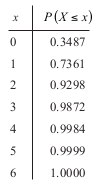
Note that tables of cumulative binomial probabilities are available.
For example, B(10, 0.1) has entries as shown opposite.
So if X is distributed B(10, 0.1) , then P(X ≤ 3) = 0.9872.
But
| P(X = 3) | = P(X ≤ 3) − P(X ≤ 2) |
| = 0.9872 − 0.9298 | |
| = 0.0574 |
This figure may be inaccurate in the last digit as it has come from two numbers which have both been rounded. Using tables usually saves having to do several calculations and the benefit is considerable in cases such as Y ~ B(30, 0.1) when the value of quantities like P(Y ≤ 8) are needed.
Exercises
